
Table of Contents
Introduction
Support vector machines (SVM) is a useful tool in supervied classification learning to analyze data. I will be discussing two main methods for SVM calculations, linear and RBF kernel, in this post.
SVM Details
SVM relies on calculating a separating hyperplane that maximizes its distance from the closest points (which are the support vectors). This allows us to derive the classification separation that offers us the greatest confidence in our classification results.
Linear SVM does this by linear classification hyperplanes separating the various data groups. Kernel methods make use of dimensionality projection in transforming non-linear classification problems into systems with linear solutions. An example is below:
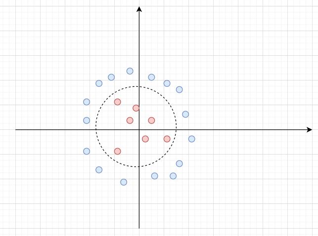
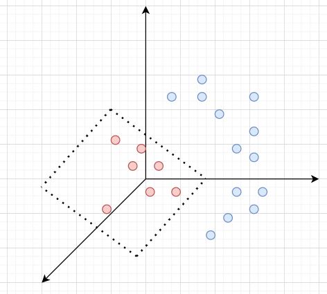
We have a classification problem with a non-linear solution on a 2 dimensional plane. However, we can raise this to 3 dimensions, resulting in the below linear classification:
Defining the problem
We will conduct a classification on the Fisher Iris data set. It is the same data used in the multiclass and k-means classification post here.
Due to the nature of SVM classification, we will need to conduct a multiclass comparison between the three classes of Iris, namely Setosa, Versicolor and Virginica. For each class, we will conduct a one-vs-rest SVM classification, and then for cross validation predictions, we will compare the SVM output in a soft-max function, picking the class for each sample that has the highest probability.
80% of the data will be used for training, and 20% for cross validation. This is evenly distributed across the three classes.
We will be conducting the SVM on all four features in the dataset. However, we will visualize the data on only 3 dimensions, as 4th dimension visualization is difficult to interpret.
Calculations
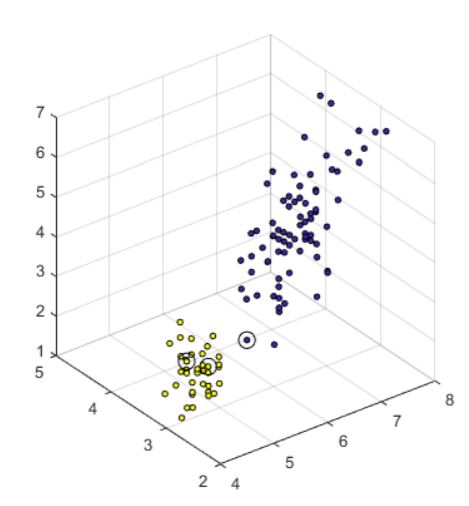
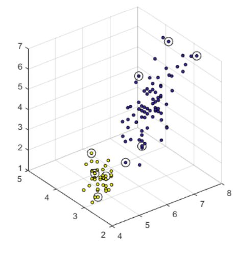
Linear SVM gives us strong training set predictions. A sample of the support vector calculations is shown below for Setosa, with Setosa being the yellow datapoints, the others being blue, and each support vector circled in black.
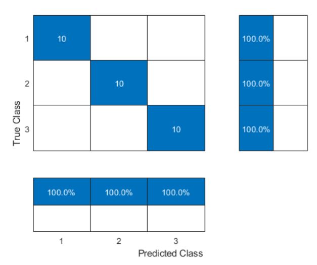
Cross validation confusion matrix is below, demonstrating 100% model accuracy in linear classification with SVM:
RBF kernel SVM also gives us similar predictions. sample of the support vector calculations is shown below for Setosa.
We note that while the results are similar, the support vectors chosen are very different due to dimensionality transformations.
The confusion matrix likewise shows 100% accuracy in the model.
Code
The full self written MATLAB code and dataset used is available on the github page for the project.
Takeaways
SVM is another method to approach classification problems. Data visualization is important in deciding if linear or kernel based SVM would perform better.