
Table of Contents
Introduction
The goal of this exercise is to investigate the power of parallel computing in performing machine learning algorithms and assisting with speeding up calculations. We will define a problem, and then compute it using parallel vs. serial computing for various samples of size n, to investigate the relative speedup and efficiency.
Parallel Computing
Parallel computing refers to the ability of computing programss to perform simultaneous computations on parallel processors. Ideally, running a calculation that is naturally parllelizable should result in N times faster calculation, where N is the number of parallel cores. This is of course influenced by the way the code is set up, if there are any dependent tasks, and costs involved with transmission of information.
Defining The Problem
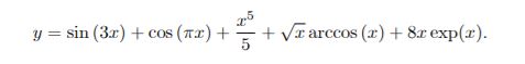
We define our x value as being randomly drawn from a uniform distribuion on [0,1], and our y value per the below formula:
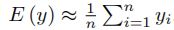
For each value of x drawn, we calculate a corresponding y value. We then approximate the expectation of y using a Monte Carlo integration method, where:
We attempt to calculate this problem for various numbers n of x, ranging from 1 to 10^8. The time taken to calculate the problem is compared between serial and parallel computing methods through speedup and efficiency factors.
Speedup at a certain n is defined as time taken for serial computation divided by time taken for parallel computation at that n.
Efficiency at a certain n is defined as time taken for serial computation divided by time taken for parallel computation at that n, divided by the number of cores used.
Comparison
The below graph demonstrates the speedup / efficiency comparison between serial and parallel computing on various sizes of n. From what we can see, the speedup increases as n increases for low values of n, up to a certain point where it remains roughly constant. Speedup peaks at around 3 times faster for a 4 core computer.
Efficiency on the other hand remains below 1 throughout. However, it too increases with n at low values of n up to a certain point.
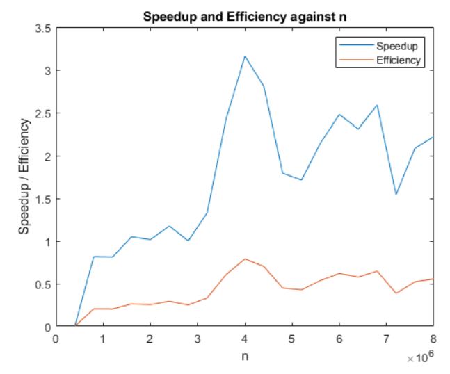
I attribute most of the fluctuations in speedup and efficiency to my old computer lagging at certain moments, which adds a degree of randomness to the results that should be discounted.
The general trend matches our expectations. At low levels of n, the time taken for information transfer between cores is large relative to total time taken, and hence both speedup and effiency are lower than they could be. At high values of n, calculation time is the majority of the time taken, and information transfer time becomes less important. Hence, speedup and effiency rise up to a point where it becomes relatively constant.
Code
The full self written MATLAB code and dataset used is available on the github page for the project.
Takeaways
I actually also attempted GPU computing as part of this project. However, this was limited by a few factors. Firstly, the GPU on my laptop is not ideal for GPU computing. Secondly, GPU code that is not optimized actually suffers greatly from information exchange costs. I was seeing calculation times for GPU code over 100 times slower than even serial computing at low n values. Hence, it stresses the importance of optimized code for parallel and GPU computing to reduce wasted calculation and information transfer time.