Data Analysis and Regression - Gradient Descent and Newton Method for Optimization

Table of Contents

1. Introduction
2. Model
3. Code
4. Take Aways

Introduction

As part of the Advanced Econometrics class, we did an exploration of Gradient Descent and Newton Method as an optimization tool for machine learning, in relation to linear and logistic regressions. In this post, I will be documenting the learning points and my key take aways from this.

Model

As part of the project, we were expected to write our own gradient descent and Newton method code to find the optimal solutions to the below set of multi-variate functions:

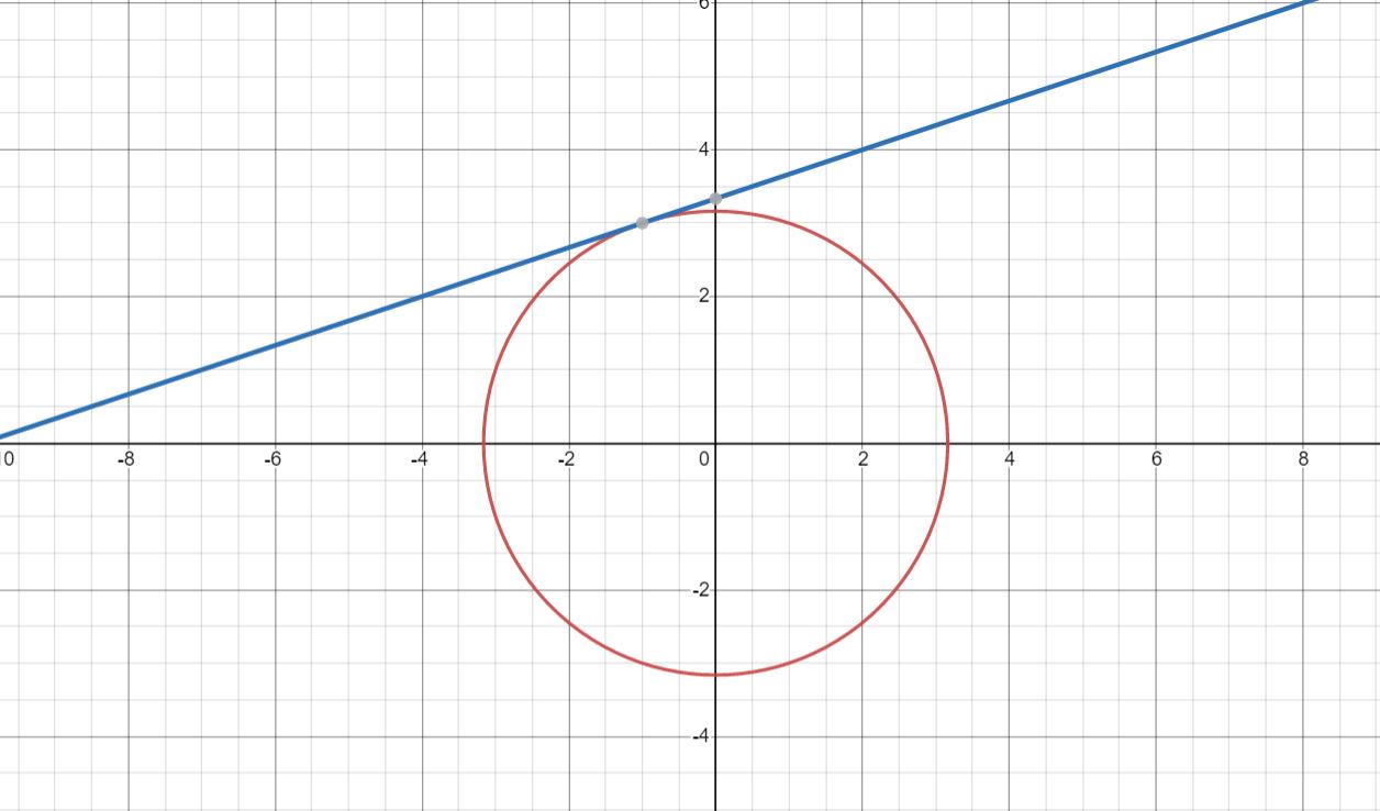
Function 1:

x^2 + y^2 = 10
x - 3y = -10

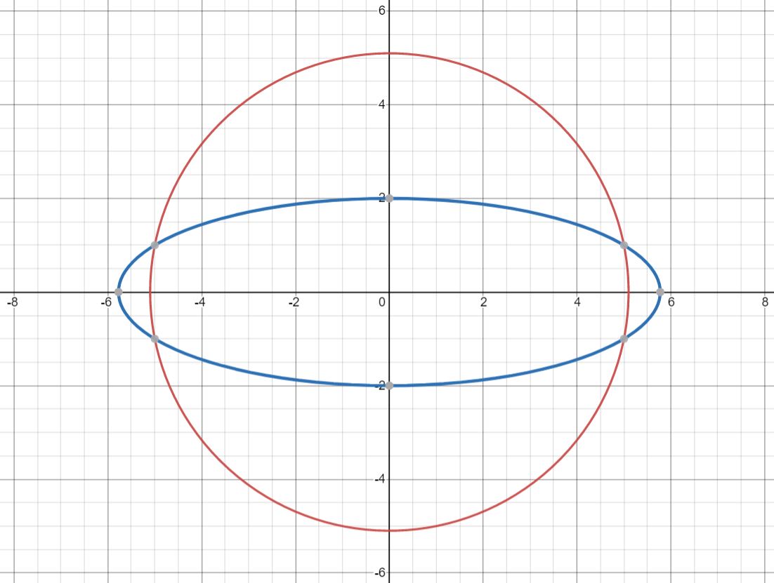
Function 2:

x^2 + y^2 = 26
3x^2 + 25y^2 = 100

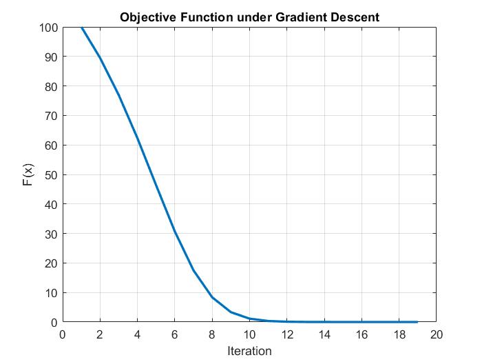
The regressions were run over 1000 iterations, with a learning rate of 0.001.

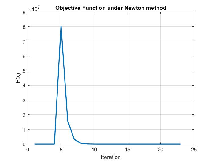
In general, the gradient descent and Newton methods arrived at the same answers as MATLAB’s own optimization functions. The number of iterations is roughly the same, although the Newton method theoretically should converge faster.

Also, it must be noted that the Newton method seems to see a divergence prior to converging to the right answer. This could be due to an issue with the learning rate, or due to the relative location of the starting guess in relation to the minimum point.

Code

The full self written MATLAB code is available on the github page for the project.

Take Aways

1. Learning rate is extremely important. High learning rates often result in divergence, while learning rates that are too low could result in extremely slow convergence.

2. Newton method seems to show a divergence prior to convergence. This could be due to the relative position of the starting guess.

3. For systems where there are more than 1 optimum point, such as in Function 2, the end result that optimization gives is dependent on the starting location. Hence, it is necessary to check multiple different starting points for all optimization routines.