Machine Learning Stochastic Descent And Minibatch Descent

Table of Contents

1. Introduction
2. Stochastic Gradient Descent
3. Minibatch Gradient Descent
4. Conventional Gradient Descent
5. Comparison

Introduction

This exercise was an investigation into different methods for running gradient optimization iterations. The investigation is around single selection stochastic descent vs. mini-batch descent vs. conventional gradient descent.

For the exercise, I generated an arbitrary set of X and Y variables following the below:

1. p random variables of length n were drawn from an N(0,1) normal distribution to act as the column vectors for our feature matrix X. A column of 1s of length n was added to this to derive X.

2. Random errors $\epsilon$ were drawn from an N(0,$\sigma^2$) normal distribution of length n. $\sigma$ is assumed be $\frac{(p+1)}{10}$

3. Y is taken to be equal to $X\theta + \epsilon$ where $\theta$ is p randomly drawn coefficients from a uniform distribution on [-1,1].

Our goal then is to estimate $\hat{\theta}$ given the generated values of X and Y. RNG seed was kept fixed for reproducability at 2021.

Cost function is standardized at $\frac{1}{2n}\sum_{i=1}^{n} (y_{i}-x_{i}\theta)^2$

Stochastic Gradient Descent

Instead of calculating the gradient on the entire training set, stochastic gradient descent involves drawing random individual samples from the training set and conducting gradient descent with that single sample, with replacement. This is then iterated as many times as necessary to derive an optimal approximation on the $\theta$ coefficients. For the purposes of this exercise, I iterated the function 10,000 times with a learning rate $\alpha$ of 0.001.

The iteration function is $\theta_{j} = \theta_{j} - \alpha((x_{i}\theta-y_{i})x_{i})$ where $x_{i}$ and $y_{i}$ denote the $i$ th row of the training set, selected randomly.

Over 10,000 iterations, we derived a final cost of 163,369 from stochastic descent. Below is a graphical example of what stochastic descent looks like on a topological function:

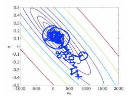
"Image credit: Serguei Maliar, Columbia University"

As shown, stochastic gradient descent takes random steps based on the probability weights of the sample distribution within the training set. Over many iterations, it converges roughly to optimal point, but with a fixed learning rate, may oscillate around the optimal point.

With a converging learning rate of, for example, $\alpha = \frac{Constant 1}{Iteration Number + Constant 2}$, we will achieve convergence that looks like the below. This is due to a decreasing emphasis on the effects of the gradient on our approximation of $\theta$ with increasing iteration count, allowing for a closer convergence to optimum.

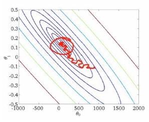
"Image credit: Serguei Maliar, Columbia University"

Minibatch Gradient Descent

Minibatch gradient descent differs from stochastic gradient descent in that instead of individual row samples, we instead select a random batch of samples of size $l < n$ where $n$ is the size of the training set.

The iteration function is $\theta_{j} = \theta_{j} - \frac{\alpha}{l}\sum_{k=1}^{l}((x^{k}\theta-y^{k})x^{k})$ where $x^{k}$ and $y^{k}$ denote the $k$ th term in the $l$ sized batch of samples selected randomly from the training set.

Final cost for minibatch gradient descent is 149,905, much lower than stochastic gradient descent.

Conventional Gradient Descent

The conventional gradient descent selected is similar to what was discussed in the Gradient Descent post.

Final cost for minibatch gradient descent is 148,312, much lower than stochastic gradient descent, and lower than minibatch, but not significantly.

Comparison

For various values of p (number of features), n (number of samples in training set) and l (size of batch) that were tested, we can see a general trend in the comparison between the three gradient descent methods.

1. Generally stochastic descent is the fastest to run, given that it calculates on individual samples instead of multiple samples or the whole training set. Minibatch gradient descent is the 2nd fastest, with conventional gradient descent being the slowest.

2. Stochastic gradient descent does not necessarily give the model with the lowest cost. This is expected as it has a high degree of randomness with its sample selection process. Without a converging learning rate $\alpha$, stochastic gradient descent may not even converge fully. Minibatch and conventional gradient descent tend to be fairly comparable, and hence the preferred gradient descent method would be minibatch due to its faster computation times. At certain levels of n and p, minibatch has a computation speed that is around 50% slower than stochastic, but almost 10 times faster than conventional gradient descent.